Tuesday, May 28, 2013

String Matching Algorithms

Some of String Matching Algorithms are :
Naïve string search algorithm
Knuth–Morris–Pratt algorithm
Boyer–Moore string search algorithm

String matching algorithm is finding all occurrences of a pattern in a text . 
Assume that the text is an array T[1 . . n] of length n and that the pattern is an array P[1 . . m] of length m.We say that pattern P occurs with shift s in text T (or, equivalently, that pattern P occurs beginning at position s + 1 in text T) if 0 <= s <=  n - m and T[s + 1 . . s + m] = P[1 . . m]
It can be useful in
   Text Editing
   Search Engine 
   Multimedia
   Network Intrusion Detection System
   Bioinformatics  and Cheminformatics and many more

Naïve string search algorithm Steps :


Knuth–Morris–Pratt algorithm :

Knuth, Morris and Pratt proposed a linear time algorithm for the string matching problem. 
A matching time of O(n) is achieved by avoiding comparisons with elements of ‘T’ that have previously been involved in comparison with some element of the pattern ‘P’ to be matched. i.e., backtracking on the text/string ‘T’ never occurs

Components of KMP algorithm

The prefix function, Π
The prefix function,Π for a pattern encapsulates knowledge about how the pattern matches against shifts of itself. This information can be used to avoid useless shifts of the pattern ‘P’. In other words, this enables avoiding backtracking on the string ‘T’.

The KMP Matcher
With string ‘T’, pattern ‘P’ and prefix function ‘Π’ as inputs, finds the occurrence of ‘P’ in ‘T’ and returns the number of shifts of ‘P’ after which occurrence is found. 


Following pseudocode computes the prefix fucnction, Π:

Compute-Prefix-Function (p)
    m := length[P]               //’P’ pattern to be matched
 Π[1] := 0 
  k := 0
 for q := 2 to m
         do while k > 0 and P[k+1] != P[q]
                       do k := Π[k]
              If P[k+1] = P[q]
                 then k := k +1
               Π[q] := k
     return  Π


Boyer-Moore Algorithm :
Developed in 1977, the B-M string search algorithm is a particularly efficient algorithm, and has served as a standard benchmark for string search algorithm ever since.
This algorithm’s execution time can be sub-linear, as not every character of the string to be searched needs to be checked.
Generally speaking, the algorithm gets faster as the target string becomes larger.

How does it work :
   Right to left scan
   Bad character rule
   Good suffix rule


Bad character rule :
Definition :
For each character x in the alphabet, let R(x) denote the position of the right-most occurrence of character x in P.  
R(x) is defined to be 0 if x is not in P

Usage
Suppose characters in P[i+1..n] match T[k+1..k+n-i] and P[i] mismatches T[k].
Shift P to the right by max(1, i - R(T[k])) places
Hopefully more than 1


Observation of Bad character rules :
Work well in practice with large alphabets like the English alphabet
Work less well with small alphabets like DNA

Strong good suffix rule :
P[i..n] matches text T[j..j+n-i] but T[(j-1) does not match P(i-1)
The rightmost non-suffix substring t’ of P that matches the suffix P[i..n] AND the character to the 
        left of t’ in P is different than P(i-1)
Shift P so that t’ matches up with T[j..j+n-i]


Monday, May 27, 2013

Searching/Sorting Algorithm Tips

Searching Algorithms :
A search algorithm is an algorithm for finding an item with specified properties among a collection of items.
It can be used for :
Database/Files.
Data structures
Graphs
String matching
Information retrieval
Elements of a search space defined by a mathematical formula or procedure(roots of equation etc.)

Pseudo Code of Recursive Binary Search :
int binary_search(int A[], int key, int imin, int imax) 
{
      // test if array is empty
     if (imax < imin): 
             // set is empty, so return value showing not found 
             return KEY_NOT_FOUND; 
     else { 
            // calculate midpoint to cut set in half 
            int imid = midpoint(imin, imax); 
            // three-way comparison 
           if (A[imid] > key) 
                     // key is in lower subset 
                    return binary_search(A, key, imin, imid-1); 
          else if (A[imid] < key)
                   // key is in upper subset
                    return binary_search(A, key, imid+1, imax); 
             else // key has been found 
         return imid; 
              } 
 }

Improvement in Binary Search Algorithm :

Binary Search takes three paths based on the key comparison: 
1)one path for less than
2)one path for greater than
3)one path for equality.
The path for equality is taken only when the record is finally matched, so it is rarely taken. Therefore it can be moved outside the search loop in the deferred test for equality version of the algorithm.

Deferred detection of equality :
int binary_search(int A[], int key, int imin, int imax) 
     // continually narrow search until just one element remains 
     while (imin < imax) {
          int imid = midpoint(imin, imax); 
           // code must guarantee the interval is reduced at each iteration 
          assert(imid < imax);
           // note: 0 <= imin < imax implies imid will always be less than imax 
          // reduce the search 
          if (A[imid] < key) 
                imin = imid + 1; 
           else imax = imid; 
          } // At exit of while: 
          // if A[] is empty, then imax < imin 
          // otherwise imax == imin 
         // deferred test for equality 
         if ((imax == imin) && (A[imin] == key)) 
                  return imin; 
         else return KEY_NOT_FOUND; 
}

How do we search in Dictionary/Telephone Booklet ?
To search on Dictionary/Telephone Booklet , we do Interpolation/extrapolation search.

Interpolation/extrapolation search :

public int interpolationSearch(int[] sortedArray, int toFind)
      // Returns index of toFind in sortedArray, or -1 if not found 
      int low = 0; 
      int high = sortedArray.length – 1,mid; 
      while (sortedArray[low] <= toFind && sortedArray[high] >= toFind) 
      { 
            mid = low + ((toFind - sortedArray[low]) * (high - low)) / (sortedArray[high] - sortedArray[low]); 
            //out of range is possible here 
           if (sortedArray[mid] < toFind) low = mid + 1; 
           else if (sortedArray[mid] > toFind) 
           // Repetition of the comparison code is forced by syntax limitations.  
          high = mid - 1; 
        else return mid; 
       } 
       if (sortedArray[low] == toFind) 
       return low; 
      else return -1; // Not found 
}

Knuth have provided the Proof of above equation : mid = low + ((toFind - sortedArray[low]) * (high - low)) / (sortedArray[high] - sortedArray[low].

Improve Selection Sort : To improve the selection sort, we use Bingo Sort. In this we skip the comparison of same elements.

bingo(array A) 
{ This procedure sorts in ascending order. } 
    begin max := length(A)-1; 
    { The first iteration is written to look very similar to the subsequent ones, but without swaps}. 
    nextValue := A[max]; 
    for i := max - 1 downto 0 do 
            if A[i] > nextValue then 
                nextValue := A[i]; 
      while (max > 0) and (A[max] = nextValue) do 
            max := max - 1; 
       while max > 0 do begin 
          value := nextValue; 
          nextValue := A[max]; 
      for i := max - 1 downto 0 do 
           if A[i] = value then begin 
               swap(A[i], A[max]); 
              max := max - 1; 
           end else if A[i] > nextValue then 
           nextValue := A[i]; 
       while (max > 0) and (A[max] = nextValue) do 
               max := max - 1; 
       end; 
end;

Improvement in Bubble Sort : Stop at the sorting process at that iteration where swapping b/w numbers didn't occur.
Pseudo Code of Bubble Sort Improvement :
procedure bubbleSort( A : list of sortable items ) 
    repeat 
       swapped = false 
      for i = 1 to length(A) - 1 inclusive do:
          /* if this pair is out of order */ 
         if A[i-1] > A[i] then 
             /* swap them and remember something changed */ 
             swap( A[i-1], A[i] ) 
            swapped = true 
         end if 
       end for 
     until not swapped 
end procedure

Improvement in Insertion Sort :Insertion sort can be improve by using binary search in insertion sort at the time of searching the location of swap element.
That's variant of insertion sort also called as Binary Insertion Sort.


BinaryInsertionSort (int a[], int n) 
{
      int ins, i, j,tmp; 
      for (i = 1; i < n; i++) 
      { 
              ins = BinarySearch (a, 0, i, a[i]); 
              if (ins < i) 
              { 
                      tmp = a[i]; 
                     for (j = i - 1; j >= ins; j--) 
                          a[j + 1] = a[j]; 
                     a[ins] = tmp; 
                }  
        }
 } 

Comparison of Selection Sort, Bubble Sort and Insertion Sort

Where should we use Insertion Sort instead of Selection Sort and Bubble Sort? :
  Where the data set have most of the elements are sorted order. Then we should use insertion sort.

Where should we use Selection Sort  or Bubble instead of Insertion sort ?
     Where the space requirement is less like as embedded programming, there we should use selection sort/bubble sort. Because in that shifting of element doesn't occur like as insertion sort. 
  

Quicksort is a divide and conquer algorithm :


Steps are:
 Step 1 : Pick an element, called a pivot, from the list.

 Step 2 : Reorder the list so that all elements with values less than the pivot come before the pivot, while all elements with values greater than the pivot come after it (equal values can go either way). After this partitioning, the pivot is in its final position. This is called the partition operation.

Step 3 : Recursively sort the sub-list of lesser elements and the sub-list of greater elements.

Lets take the example of Quick Sort


Repeat above 4 steps till then small_index cross the big index.


A single quicksort call involves O(n) work plus two recursive calls on lists of size n/2, so the recurrence relation is :T(n) = O(n) + 2T(n/2)
The master theorem tells us that T(n) = O(nlogn)

Merge Sort :
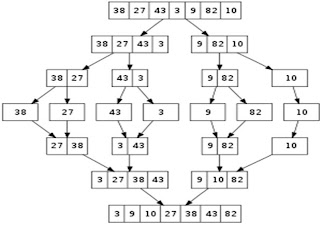
Conceptually, a merge sort works as follows :
Step 1: Divide the unsorted list into n sublists, each containing 1 element (a list of 1 element is considered sorted).
Step 2: Repeatedly merge sublists to produce new sublists until there is only 1 sublist remaining. This will be the sorted list


If the running time of merge sort for a list of length n is T(n), then the recurrence T(n) = 2T(n/2) + n follows from the definition of the algorithm (apply the algorithm to two lists of half the size of the original list, and add the n steps taken to merge the resulting two lists). 
The closed form follows from the master theorem T(n) = O(n) + 2T(n/2)
The master theorem tells us that T(n) = O(nlogn)

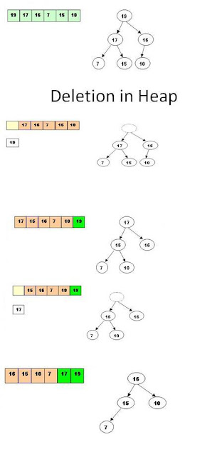
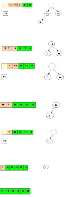
Heap Sort :
Steps are :
   Step 1 : Consider the values of the elements as priorities and build the heap tree.
   Step 2 : Start deleteMin operations, storing each deleted element at the end of the heap array.

Heap Construction and Deletion :


Comparison Tips :
Quicksort is typically somewhat faster due to better cache behavior and other factors, but the worst-case running time for quicksort is O(n2), which is unacceptable for large data. 
Merge sort requires auxiliary space according to value of n, but heapsort requires only a constant amount.
Heapsort is not a stable sort; merge sort is stable.
Merge sort parallelizes well and can achieve close to linear speedup with a trivial implementation; heapsort is not an obvious candidate for a parallel algorithm.
Merge sort is used in external sorting; heapsort is not. Locality of reference is the issue.


Radix Sort :
Steps are :
Step 1 : Take the least significant digit (or group of bits, both being examples of radices) of each key.
Step 2 : Group the keys based on that digit, but otherwise keep the original order of keys. (This is what makes the LSD radix sort a stable sort).
Repeat the grouping process with each more significant digit.

The sort in step 2 is usually done using bucket sort or counting sort, which are efficient in this case since there are usually only a small number of digits.
 Example :
Original, unsorted list: 170, 45, 75, 90, 802, 24, 2, 66
Sorting by least significant digit (1s place) gives: 
       170, 90, 802, 2, 24, 45, 75, 66
    [*Notice that we keep 802 before 2, because 802 occurred before 2 in the original list, and similarly for   pairs 170 & 90 and 45 & 75.]
Sorting by next digit (10s place) gives: 
     802, 2, 24, 45, 66, 170, 75, 90
    [*Notice that 802 again comes before 2 as 802 comes before 2 in the previous list.]
Sorting by most significant digit (100s place) gives:
    2, 24, 45, 66, 75, 90, 170, 802

Radix sort takes O(k*n) time

Shell Sort :

Shellsort is a multi-pass algorithm. Each pass is an insertion sort of the sequences consisting of every h-th element for a fixed gap h (also known as the increment). This is referred to as h-sorting.
An example run of Shellsort with gaps 5, 3 and 1 is shown below :


Generally Gap Sequence is


It needs relatively short code and does not use the call stack. Therefore  it use in embedded systems instead of quick sort.

Sunday, May 26, 2013

Basic Math in Algorithms

First time when we used the Algorithm ? :
         Isn’t when we started to visualize the things?
         Isn’t when we started to speak?
         Isn’t when we started to identify the words?
         Isn’t when we started to learn rules for Addition , Multiplication etc?
         Is algorithm related to only computer science?

Mathematics in Algorithms :
Mathematical analysis of algorithms occupies a central position in computer science; reasoning about algorithms independently of the specific devices  on which they run can yield insight into general design principles and fundamental constraints on computation.
Mathematics is the core part of Algorithms.

Such as in statistics / probability (i.e. for scientific and financial programming),  abstract algebra and number theory (i.e. for cryptography).
Recently Google Published  Mathematics at Google

Vectors and Matrix :
    Vectors  Application:
          Machine learning, a supervised learning method used for classification.(Feature Vector)
          Cryptography(Initialization vector (IV))
          Vector graphics (VML  : XML for to produce vector graphics)
    Matrix Application :
          Eigen Vector
          Linear Equations

  Vectors :
     Vectors quantities are physical quantities that have both magnitude and direction
     The displacement vector shown below :


The triple of real numbers d1x=(x2-x1), d1y=(y2-y1), d1z=(z2-z1) are called the Cartesian components of displacement vector d1.

 Vector Addition is shown below :


Vector Product : Product of two vector computed as :


It also called as scalar product or dot product.

Cross Product of Vector: Vector cross product is computed as :


It also called as Cross Product.

Dot product uses cos  to measure “how parallel” two vectors are (cos(00) = 1), while the cross product uses sin  to measure “how perpendicular”  they are (sin(900) = 1).


Matrix :

Basic matrix operations are :


Matrix multiplication use at so many places in m/c learning. Time Complexity of matrix multiplication is O(n3). In matrix multiplication .multiplication of each row with each column takes O(n2) and combining them takes O(n). Thats why matrix multiplication takes O(n3) time.
Strassen build algorithm with some equation through which matrix multiplication takes O(n2.807) time.


Cosine Similarity use in m/c learning to find the how much two documents are similar. In below figure cosine similarity is calculated in b/w two documents x and y as :


Eigen Vectors also use in many placed in m/c learning. It use in PCA(Principal Component Analysis) for dimension reduction regarding m/c learning. It also use for reducing term-document matrix dimension in IR(Information Retrieval).
An Eigen vector of a square matrix is a non-zero vector that, when multiplied by the matrix, yields a vector that is parallel to the original.
   
Right eigenvector : Av = λv
Left eigenvector : vA = λv

Eigen vector present by graph and matrix shown below :


Eigen vector example shown below :


In above example first is eignen vector because here Ax = λx but in second Ax != λx so second is not an eigen vector.

Eigen value calculation for eigen vector as :


From above example eigne value calculated are 3 and 4. Lets calculate eigen vector from eigen value 3 in below example as :


Probability :

Some of Common Usage in Computer Science are :
      Artificial intelligence(Bayesian Sequence Prediction)
      Machine learning(Naive Bayes Classifier)

      Game Theory(Strategy, Decision Making)

Some Basic Probabilities are :


Difference b/w mutually exclusive and independent probability is mutually exclusive happens on same experiment and independent happens on different experiment. Ex. Tossing a coin once and getting head or tail is mutually exclusive. But if tossing a coin twice and getting HH or TT is independent Probability.

Conditional Probability :
Conditional probability is the probability that an event will occur, when another event is known to occur or to have occurred. If the events are A and B respectively, this is said to be "the probability of A given B". It is commonly denoted by P(A|B).


Bayesian Probability :
Bayes' theorem (alternatively Bayes' law or Bayes' rule) is a theorem with two distinct interpretations :
1) In the Bayesian interpretation, it expresses how a subjective degree of belief should rationally change to account for evidence.
2) In the frequentist interpretation, it relates inverse representations of the probabilities concerning two events.

Bayesian interpretation : Bayes' theorem then links the degree of belief in a proposition before and after accounting for evidence.
For example, somebody proposes that a biased coin is twice as likely to land heads than tails. Degree of belief of in this might initially be 50%. The coin is then flipped a number of times to collect evidence. Belief may rise to 70% if the evidence supports the proposition.

For proposition  A and evidence B
P(A): the prior, is the initial degree of belief in  A.
P(B): the posterior, is the degree of belief having accounted for B.
P(B|A)/P(B) : represents the support  B provides for A.

Frequentist interpretation : In this probability measures a proportion of outcomes. Bayes' theorem under this interpretation is most easily visualized using tree diagrams.


Bayes Theorem  Application : Naive Bayes Classifier
A naive Bayes classifier is a simple probabilistic classifier based on applying Bayes' theorem with strong (naive) independence assumptions

Set Theory :

Some of Common Usage in Computer Science are :
Graph Theory(MST, Shortest Path)
Game Theory(set of players,  set of moves)
Artificial Intelligence(Fuzzy Set)

Some of basic operations in set theory are :

Union
Intersection
Set difference :  {2,3,4} \ {1,2,3}  ->  {4}
Symmetric difference : {1,2,3} and {2,3,4} -> {1,4}
Cartesian product
Power set

Relationships between Sets
Equality : {1, 2, 3} = {3, 2, 1} = {1, 1, 2, 3, 2, 2}
Subsets : A ⊆  B and A ⊂  B 
Disjoint : A = {even numbers} and B = {1, 3, 5, 11, 19}, then A and B are disjoint.
Venn Diagram
Truth Table

Fuzzy Set : Fuzzy set is the set where crisp boundary doesn't exist b/w set. Below the example of fuzzy set :